Activations: MNIST#
Abstract#
In this notebook we discuss tracking of activations of layers by outputs and by parameter gradients. Firstly we analyse binary classification of linearly separable data and then we proceed to examine effect of dropout layers on deep convolutional layer for classification on MNIST dataset. For a much deeper dive see Neuron Death in ANNs: detecting and troubleshooting by Malcolm Lett.
Imports#
import numpy as np
import pandas as pd
import matplotlib.pyplot as plt

import torch
import torch.nn as nn
from torch.utils.data import DataLoader, TensorDataset

RND_SEED = 42
device = torch.device('cuda' if torch.cuda.is_available() else 'cpu')
device
device(type='cuda')
Activation Lenses#
The whole idea of activation stems from the ReLU and sigmoid activations
functions being zero or near-zero for a subset of real numbers. Zeros
being multiplicatevily absorbing and additively neutral element does not
interact with linear combinations, thus not propagating any information
further. Thus a dead neuron is a neuron that does not propagate any
information for all of the samples in a training iteration (batch),
death rate is a proportion of dead neurons, activation rate is a
proportion of outputs activited thorugh a dataset pass. This idea is
represented by OutputActivation lens, on every forward pass through
a layer outputs are put to be either active or inactive; death and
activation rates are then calculated.
OutputNorm records data for all activations functions and dropout by
default. Its behavious can be configured by activation, dropout,
include and exclude flags.
If neuron is dead, i.e., its outputs are constant, it will have a zero
gradient; therefore both activation and death rate can be reconstructed
from gradients with respect to neuron’s parameters. This idea is
implemented in ParameterGradientActivation lens. Note that it does
not hook onto a module, but on parameter tensors, and PyTorch allows to
hook only onto non-lazy tensors, hence lazy modules’ gradients (such as
nn.LazyLinear) cannot be tracked by this lens.
ParameterGradientActivation records data for all layer that have all
of the parameters listed in parameters initialization arguments,
default are "weight" and "bias".
Both plots allow for warning plot that plots minimal activation rate and maximal death rate accross all layers (and parameters).
It is common to implement activation functions as a functional calls to
torch.nn.functional, that way no output data can be captured using
callbacks, ParameterGradientActivation then might help you examine
your network.
Let us define the inspector with those lenses.
from monitorch.inspector import PyTorchInspector
from monitorch.lens import LossMetrics, OutputActivation, ParameterGradientActivation

loss_fn = nn.CrossEntropyLoss()

inspector = PyTorchInspector(
    lenses = [
        LossMetrics(
            loss_fn=loss_fn,
            separate_loss_and_metrics=False,
            metrics=['val_accuracy']
        ),
        OutputActivation(),
        ParameterGradientActivation()
    ]
)
We will also define generic functions for training and validation.
def train_one_epoch(model, loss_fn, optimizer, train_dataloader, device=device):
    """ Trains model through dataset one time. """
    for data, label in train_dataloader:
        data = data.to(device)
        label = label.to(device)
        optimizer.zero_grad()
        pred = model(data)
        loss = loss_fn(pred, label)
        loss.backward()
        optimizer.step()

@torch.no_grad
def validate_one_epoch(model, loss_fn, val_dataloader, device=device):
    """ Validates through given dataset. """
    correctly_classified = 0
    n_samples = 0
    for data, label in val_dataloader:
        data = data.to(device)
        label = label.to(device)
        pred = model(data)
        loss = loss_fn(pred, label)
        n_samples += data.shape[0]
        correctly_classified += pred.argmax(dim=1).eq(label).float().sum().item()
    return correctly_classified / n_samples
2D Examples#
Activation rate can be seen as a measure of entropy of a layer, because task-relative informative features requires model to differentiate more complex and less common patterns. A notorious example would be that first layers of convolutional networks learn to distinguish between lines and angles, while the last can detect parts of face.
Death rate on the other hand can be interpreted as a measure of layer’s overcapacity under given architecture. Gradient-based optimization methods are well-known to find the easiest solution for a problem, sadly sometimes the easiest solution is to kill a neuron.
To illustrate our take we will train highly overparameterized network for a linearly separable case.
Let us define function for further ease of use.
def plot_decision_boundary(model, X, y, ax=None, resolution=0.02):
"""
Plots decision boundary for a binary classifier.
model: trained PyTorch model
X: torch.Tensor or np.ndarray of shape (N, 2)
y: torch.Tensor or np.ndarray of shape (N,) or (N,1)
"""
if ax is None:
fig, ax = plt.subplots()
# Convert tensors to numpy if needed
if torch.is_tensor(X):
X = X.detach().cpu().numpy()
if torch.is_tensor(y):
y = y.detach().cpu().numpy()
# Determine grid range
x_min, x_max = X[:, 0].min() - 1, X[:, 0].max() + 1
y_min, y_max = X[:, 1].min() - 1, X[:, 1].max() + 1
xx, yy = np.meshgrid(np.arange(x_min, x_max, resolution),
np.arange(y_min, y_max, resolution))
# Prepare grid for prediction
grid = np.c_[xx.ravel(), yy.ravel()]
grid_tensor = torch.tensor(grid, dtype=torch.float32)
# Get predictions
model.eval()
with torch.no_grad():
preds = model(grid_tensor)[:, 1].cpu().numpy()
Z = (preds > 0.5).astype(int) # binary mask
Z = Z.reshape(xx.shape)
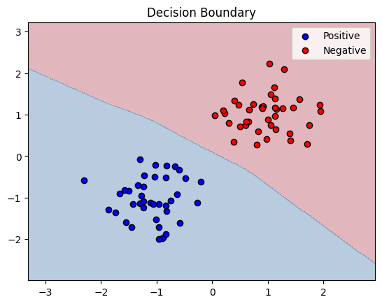
# Plot decision boundary
ax.contourf(xx, yy, Z, alpha=0.3, cmap=plt.cm.RdBu)
# Plot original points
ax.scatter(X[y==1, 0], X[y==1, 1], c='b', edgecolor='k', label="Positive")
ax.scatter(X[y==0, 0], X[y==0, 1], c='r', edgecolor='k', label="Negative")
ax.legend()
ax.set_title("Decision Boundary")
plt.show()
def make_dataloaders(pos, neg):
X = np.vstack((pos, neg))
y = np.hstack((np.ones(len(pos)), np.zeros(len(neg))))
X_tensor = torch.tensor(X, dtype=torch.float32)
y_tensor = torch.tensor(y, dtype=torch.long)
full_dataset = TensorDataset(X_tensor, y_tensor)
# Split into train and validation (e.g., 70% train / 30% val)
train_size = int(0.7 * len(full_dataset))
val_size = len(full_dataset) - train_size
train_dataset, val_dataset = torch.utils.data.random_split(full_dataset, [train_size, val_size],
generator=torch.Generator().manual_seed(RND_SEED))
train_loader = DataLoader(train_dataset, batch_size=8, shuffle=True)
val_loader = DataLoader(val_dataset, batch_size=8, shuffle=False)
return train_loader, val_loader
We will create two 2D populations both coming from a scaled gaussian distribution with different means.
np.random.seed(RND_SEED)
pos = np.random.standard_normal(size=(40, 2))*0.5 -1
neg = np.random.standard_normal(size=(40, 2))*0.5 +1
X = np.vstack((pos, neg))
y = np.hstack((np.ones(len(pos)), np.zeros(len(neg))))
plt.scatter(pos[:, 0], pos[:, 1], color='b')
plt.scatter(neg[:, 0], neg[:, 1], color='r')
train_lin_loader, validate_lin_loader = make_dataloaders(pos, neg)
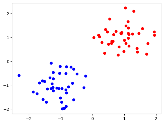
We see that data is clearly linearly separable, therefore a 3-parameter 1-layer neural network (logistic regression) would be able to learn to classify these data perfectly. Instead we will define a model with additional layer with 16 neurons, pumping number of parameters to be over three hundread.
from collections import OrderedDict

model = nn.Sequential(OrderedDict([
    ('lin1', nn.Linear(2, 16)),
    ('relu1', nn.ReLU()),

    ('lin2', nn.Linear(16, 16)),
    ('relu2', nn.ReLU()),

    ('lin3', nn.Linear(16, 2)),
    ('softmax', nn.Softmax(dim=1))
])).to(device)
inspector.attach(model)
optimizer = torch.optim.Adam(model.parameters())

N_EPOCH = 50
for epoch in range(N_EPOCH):
    train_one_epoch(model, loss_fn, optimizer, train_lin_loader)
    val_acc = validate_one_epoch(model, loss_fn, validate_lin_loader)
    inspector.push_metric('val_accuracy', val_acc)
    inspector.tick_epoch()

fig = inspector.visualizer.show_fig()
plot_decision_boundary(model.cpu(), X, y)
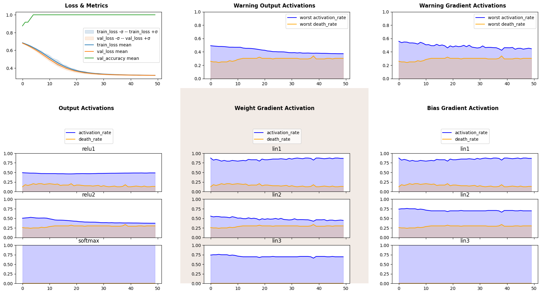
We see that both gradient and output death rates of the second (redundant) layer are high, though they do not converge to give minimal possible result of 81.5%, where the second layer would effectively have 2 neurons.
MNIST#
Now we will show how activations work on an example where it is not as easy to come up with correct number of parameters and how one could influence model’s activations.
Firstly we will download MNIST dataset.
from torchvision.datasets import MNIST
import torchvision.transforms as transforms

transform = transforms.Compose([
        transforms.ToTensor(),
        transforms.Normalize((0.5,), (0.5,))
])

trainset = MNIST(
    './data',
    download=True,
    train=True,
    transform=transform
)

testset = MNIST(
    './data',
    download=True,
    train=False,
    transform=transform
)
BATCH_SIZE = 256
trainloader = torch.utils.data.DataLoader(trainset, batch_size=BATCH_SIZE, shuffle=True, num_workers=2)

validateloader = torch.utils.data.DataLoader(testset, batch_size=BATCH_SIZE, shuffle=False, num_workers=2)
100%|██████████| 9.91M/9.91M [00:00<00:00, 57.3MB/s]
100%|██████████| 28.9k/28.9k [00:00<00:00, 1.73MB/s]
100%|██████████| 1.65M/1.65M [00:00<00:00, 14.8MB/s]
100%|██████████| 4.54k/4.54k [00:00<00:00, 6.47MB/s]
We will define custom convolutional network with controllable dropout parameter between two convolutional layers, convolutional and fully connected part and before the output layer.
class CNN(nn.Module):

    def __init__(self, dropout=(0, 0, 0)):
        super().__init__()
        self.conv = nn.Sequential(OrderedDict([
            ('conv1', nn.Conv2d(1, 64, kernel_size=7, padding='same')),
            ('pool1', nn.MaxPool2d(kernel_size=7)),
            ('relu1', nn.ReLU()),

            ('dropout', nn.Dropout(dropout[0])),

            ('conv2', nn.Conv2d(64, 128, kernel_size=4)),
            ('relu2', nn.ReLU()),
        ]))

        self.dense = nn.Sequential(OrderedDict([
            ('dropout1', nn.Dropout(dropout[1])),
            ('lin1',  nn.Linear(128, 32)),
            ('relu1', nn.ReLU()),

            ('dropout2', nn.Dropout(dropout[2])),
            ('lin2',    nn.Linear(32, 10)),
            ('softmax', nn.Softmax(dim=1))
        ]))

    def forward(self, X):
        t = torch.flatten(self.conv(X), start_dim=1)
        return self.dense(t)
We will also use an early stopping mechanism.
class EarlyStopper:
    def __init__(self, patience : int = 5, eps : float = 1e-3):
        self.loss = float('+inf')
        self.timer = 0
        self.eps = eps
        self.patience = patience

    def __call__(self, new_loss : float) -> bool:
        if self.loss - new_loss > self.eps:
            self.loss = new_loss
            self.timer = 0
            return False
        self.timer += 1
        return self.timer >= self.patience
Finally let us train a network without dropout and see its activation and death rates.
from tqdm import trange
model = CNN().to(device)

stopper = EarlyStopper()
inspector.attach(model)
optimizer = torch.optim.Adam(model.parameters())

N_EPOCH = 50
for epoch in trange(N_EPOCH):
    train_one_epoch(model, loss_fn, optimizer, trainloader)
    val_acc = validate_one_epoch(model, loss_fn, validateloader)
    inspector.push_metric('val_accuracy', val_acc)
    inspector.tick_epoch()
    if stopper(inspector.lenses[0].loss(train=False)):
        break

fig = inspector.visualizer.show_fig()
44%|████▍ | 22/50 [04:06<05:13, 11.20s/it]
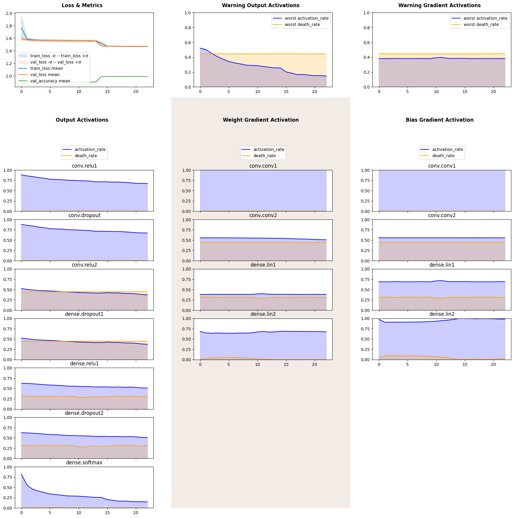
Our network has reached impressive accuracy and at the same time second convolutional and first dense layers are half dead. Another peculiar feature of this plot is a steady decline of output activation as model learns to distinguish between digits. It is even more interesting with a softmax layer, as its activation rate falls steadily and reaches approximately 10%, coinciding with the last elbow on a loss and metrics plot. 10% activation is exactly one output of softmax layer being non-zero, thus predicting correct digit.
Let us now train the very same network, but heavily regulirize half dead layers and put a weak constrain on the output layer.steadily
from tqdm import trange
model = CNN(dropout=(0.5, 0.5, 0.2)).to(device)

stopper = EarlyStopper()
inspector.attach(model)
optimizer = torch.optim.Adam(model.parameters())

N_EPOCH = 50
for epoch in trange(N_EPOCH):
    train_one_epoch(model, loss_fn, optimizer, trainloader)
    val_acc = validate_one_epoch(model, loss_fn, validateloader)
    inspector.push_metric('val_accuracy', val_acc)
    inspector.tick_epoch()
    if stopper(inspector.lenses[0].loss(train=False)):
        break

fig = inspector.visualizer.show_fig()
52%|█████▏ | 26/50 [04:44<04:22, 10.94s/it]
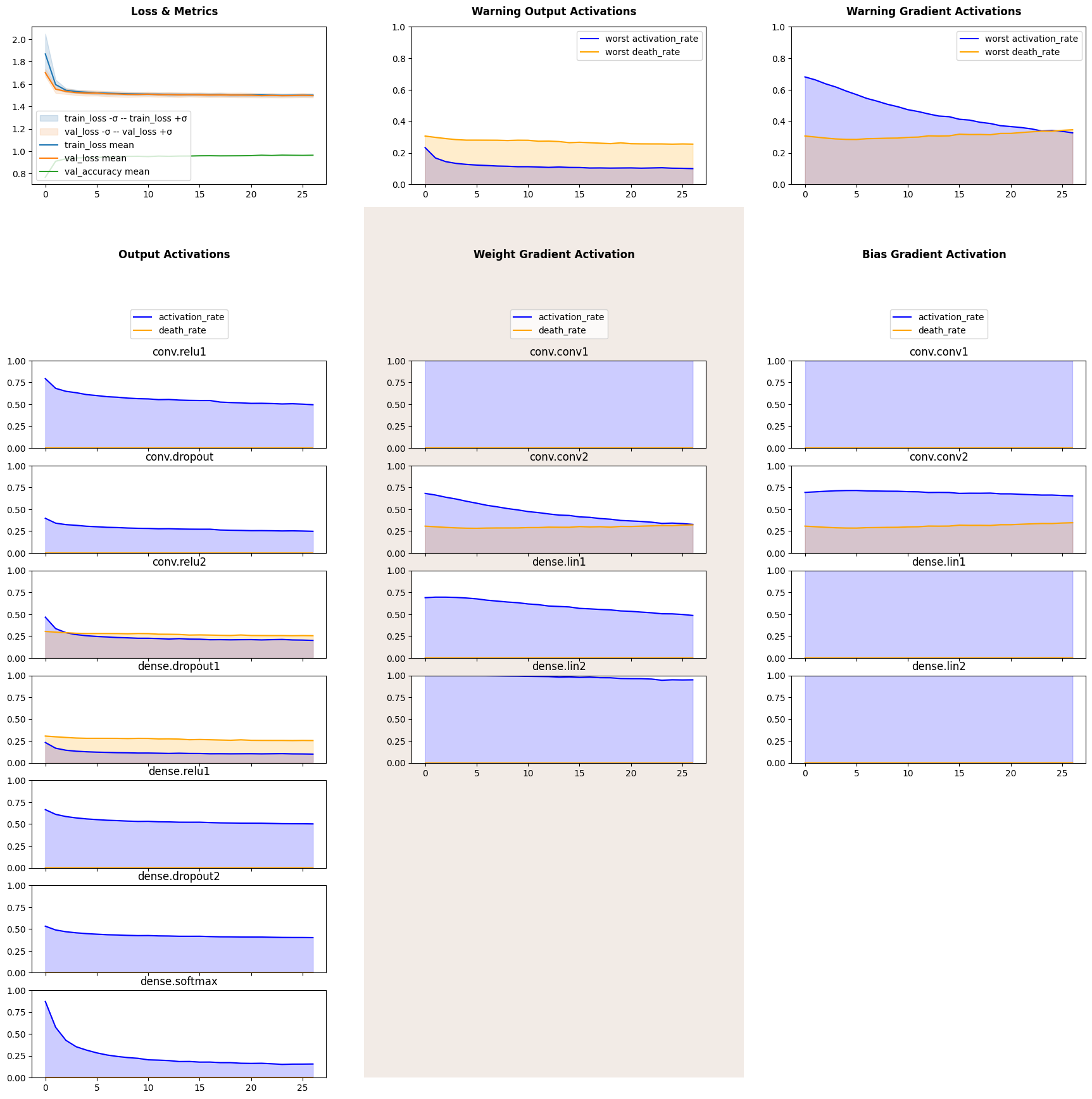
Firsly we see a that the first dense layer had almost no dead gradient, as well as, its activation function stopped producing dead outputs. Both activations and death rate of the second convolutional layer declined. Loss plots show less variance and softmax activation rate declined smoother with no hard elbows. All of that is a result of dropout reducing effective size of a model and its variance.
What to Look for#
Keep death rates low possible using dropout, dead neuron does not contribute to network at all. Occasionally dropped out neuron helps to generalize.
Output (ReLU) and gradient activations start at roughly 50% and 100% activations. Layers closer to the output should drive their activation rates lower, because they need to accept and reject more often.
Next Steps#
Read an article by Malcolm Lett.
Take a look at other demonstration notebooks and documentation.
Experiment with dropout at different parts of network.
Find what activation flavour fits your codebase and habits best.